Linear Programming¶

Colab notebook

Objectives of business decisions frequently involve maximizing profit or minimizing costs. Linear programming uses linear algebraic relationships to represent a firm’s decisions given a business objective and resource constraints. Steps in application:

Identify the problem as solvable by linear programming
Formulate a mathematical model of the unstructured problem
Solve the model

The model has multiple components:

Decision variables - mathematical symbols representing levels of activity by the firm
Objective function - a linear mathematical relationship describing an objective of the firm, in terms of decision variables - this function is to be maximized or minimized
Constraints - requirements or restrictions placed on the firm by the operating environment, stated in linear relationships of the decision variables
Parameters - numerical coefficients and constants used in the objective function and constraints

To make things more concrete, let’s consider an example:

The Factory Problem¶

A business manager develops a production plan for a factory that produces chairs and tables. The factory wants to sell a chair for $40 and a table for $50. There are two critical resources in the production of chairs and tables: wood (measured in m$^2$) and labor (measured in hours per week). At the beginning of each week, there are 40 units of wood and 50 units of labor available.

The manager estimates that

one chair requires 1 unit of wood and 4 units of labor, while
one table requires 2 units of wood and 3 units of labor.

product	profit ($/unit)	wood (m$^2$/unit)	labor (hour/unit)
chair	40	1	2
table	50	4	3

The marketing department has told the manager that ALL chairs and tables can be sold.

Problem statement: what is the production plan that maximizes total revenue given the constraints?

If the factory produces $x_1$ chairs, then since each chair generates $40, the total revenue generated by the production of chairs is $40x_1$. Similarly, the total revenue generated by the production of tables is $50x_2$. Consequently, the total revenue generated by the production plan can be determined by the following equation:

\[ \text{total revenue per week} = 40x_1 + 50x_2. \]

The production plan is constrained by the amount of resources available per week. How do we ensure that the production plan does not consume more wood or labor than the amount available?

If we decide to produce $x_1$ number of chairs, then the total amount of wood consumed by the production of chairs is $1x_1$ m$^2$. Similarly, if we decide to produce $x_2$ number of tables, then the total amount of wood consumed by the production of tables is $2x_2$ m$^2$. Hence, the total consumption of wood by the production plan determined by the values of $x_1$ and $x_2$ is $1x_1 + 2x_2$ m$^2$. However, the consumption of wood by the production plan cannot exceed the amount of wood available. We can express these ideas in the following constraint:

\[ 1x_1 + 2x_2 \le 40. \]

Similarly, we can formulate the constraint for labor resources per week. The total amount of labor resources consumed by the production of chairs is 4 labor units multiplied by the number of chairs produced that is $4x_1$ hours. The total amount of labor resources consumed by the production of tables is 3 labor units multiplied by the number of tables produced that is $3x_2$ hours. Therefore, the total consumption of labor resources by the production plan determined by the values of $x_1$ and $x_2$ is $4x_1 + 3x_2$ hours. This labor consumption cannot exceed the labor capacity available. Hence, this constraint can be expressed as follows:

\[ 4x_1 + 3x_2 \le 120. \]

In a linear programming (LP) model we have objective (goal) and constraints that must meet. Here, the objective is to maximize the total revenue (denoted by $z$) generated by the buisness plan and constraints that limit the number of chairs and tables that can be produced. That is,

\[\begin{split} \begin{align} &\text{max}&&\\ &\qquad z=40𝑥_1 + 50𝑥_2&\quad&\text{(revenue)}\\ &\text{subject to}&&\\ &\qquad 1x_1 + 2𝑥_2 \le 40&\quad&\text{(wood, m$^2$)}\\ &\qquad 4𝑥_1 + 3𝑥_2 \le 120&\quad&\text{(labor, hours)}\\ &\qquad x_1, x_2 \ge 0&\quad&\text{(non negativity)}\\ \end{align} \end{split}\]

where $𝑥_1$ is a decision variable that represents the number of chairs to produce, and $𝑥_2$ is a decision variable that represents the number of tables to produce.

Abstraction of factory problem allows us to generalize the model. That is, we are able to change the values of the parameters without changing the model structure:

\[\begin{split} \begin{align} &\text{max}\\ &\qquad z=c_1𝑥_1 + c_2𝑥_2&\quad&\text{(revenue)}\\ &\text{subject to}\\ &\qquad a_{1,1}x_1 + a_{1,2}𝑥_2 \le b_1&\quad&\text{(wood, $m^2$)}\\ &\qquad a_{2,1}𝑥_1 + a_{2,2}𝑥_2 \le b_2&\quad&\text{(labor, hours)}\\ &\qquad x_1, x_2 \ge 0&\quad&\text{(non-negativity)}\\ \end{align} \end{split}\]

where $c_1=40$, $c_2=50$, $a_{1,1}=1$, $a_{1,2}=2$, $a_{2,1}=4$, $a_{2,2}=3$, $b_1=40$, and $b_2=120$. Summation notation allows us to write the above set of equations in more concise form:

\[\begin{split} \begin{align} &\text{max}\\ &\qquad z=\sum_{i=1}^{n} c_i x_i \\ &\text{subject to} \\ &\qquad \sum_{j=1}^{m} a_{i,j} x_j \le b_i, \quad(\forall i = 1,2,.. m) \\ &\qquad x_i \ge 0, \quad(\forall i = 1,2,.. n). \\ \end{align} \end{split}\]

where $n$ is the number of decision variables (here $n=2$), and $m$ is the number of constraining resources (here $m=2$). In example,

\[\begin{split} \begin{align} &\text{max}\\ &z=\sum_{i=1}^{n} c_i x_i= c_1x_1+c_2x_2=40x_1+50x_2,\\ &\text{subject to} \\ &\sum_{j=1}^{m} a_{i,j} x_j = \left\{ \begin{array}{cl} a_{1,1}x_1+a_{1,2}x_2&\le b_1&\Rightarrow 1x_1+2x_2&=40, \\ a_{2,1}x_1+a_{2,2}x_2&\le b_2&\Rightarrow 4x_1+3x_2&=120, \end{array} \right.\\ &x_1\ge 0, x_2\ge 0.\\ \end{align} \end{split}\]

Another way of writing this is using a matrix form:

\[\begin{split} \begin{align} &\text{max}\\ &\qquad z=\mathbf{c}^T\mathbf{x} \\ &\text{subject to}\\ &\qquad\mathbf{A}\mathbf{x} \le \mathbf{b},\\ &\qquad\mathbf{x} \ge 0.\\ \end{align} \end{split}\]

Here,

\[\begin{split} \begin{align} \mathbf{c}&=(c_1,c_2)=(40,50),\\ \mathbf{x}&=(x_1,x_2),\\ \mathbf{b}&=(b_1,b_2)=(40,120), \\ \end{align} \end{split}\]

and

\[\begin{split}\mathbf{A} = \begin{pmatrix} a_{1,1} & a_{1,2} \\ a_{2,1} & a_{2,2} \end{pmatrix} = \begin{pmatrix} 1 & 2 \\ 4 & 3 \end{pmatrix}. \end{split}\]

Lastly, in a one-line format:

\[\begin{split} {\displaystyle \max\{\,\mathbf {c} ^{\mathrm {T} }\mathbf {x} \mid \mathbf {x} \in \mathbb {R} ^{n}\land A\mathbf {x} \leq \mathbf {b} \land \mathbf {x} \geq 0\,\}},\\ \end{split}\]

where $\land$ symbolizes AND.

In operation research, objective functions are maximized or minimized. For example, maximizing revenue or minimizing cost.

Constraints typically involve inequalities:

$\le$ constraints are typically considered for supply constraints that can’t exceed some threshold
$\ge$ constraints are typically used to model demand requirements where we want to ensure that at least a certain level is satisfied
$=$ constraints are used when we want to match exactly certain activities with a given requirement

A solution can be feasible or infeasible. A feasible solution does not violate any of the constraints, while an infeasible solution violates at least one of the constraints. In example, for the Factory example, $\mathbf{x}=(5,10)$ is feasible, while $\mathbf{x}=(10,20)$ is not.

Graphical Solution of Linear Programming Models¶

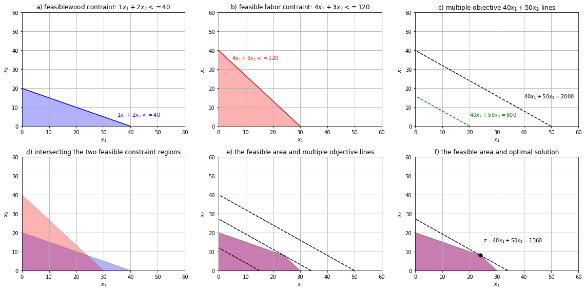
The graphical solution is limited to LP models containing only two decision variables. Graphical methods illustrate how a solution for a linear programming problem is obtained.

Panel a) of the figure below shows the region of the wood constraint $1x_1+2x_2 <= 40$ using the fact that the decisions variables are non-negative. This is the feasible area that contains the possible solutions for the decisions variables. Panel b) shows the region of the labor constraint $4x_1+3x_2 <= 120$, again, using the fact that the decisions variables are non-negative.

The goal is to maximize the objective $40x_1+50x_2$. In panel c) we show multiple lines for the various values that the objective can take.

The two constraints must meet simultaneously, and so on panel d) we intersect both constraints, and the resulting common area is the new feasible area that is considered in this problem. Panel e) shows multiple objective values with respect to the new feasible region. In linear programming, the feasible region is called a polyhedron. Panel f) is the outcome of the graphical method by which we identify the optimal solution $(x_1,x_2)=(24,8)$ to the problem. At this point, the objective is maximized with $z=\$1360$ and satisfies all the constraints of the question.

Hence, the optimal solution point is the last point the objective function touches as it leaves the feasible solution area.

import numpy as np
%matplotlib inline
import matplotlib.pyplot as plt
from matplotlib.patches import Polygon

plt.figure(figsize=(16,8))
#-------------------
plt.subplot(2,3,1)
plt.plot([40,0],[0,20],'-b')
plt.text(35,5, '$1x_1+2x_2 <= 40$', color='b')
P = np.array([
        [0, 40, 0],
        [0, 0, 20]
    ])
plt.gca().add_artist(Polygon(P.T, alpha=0.3, color="b"))
plt.grid()
plt.axis([0, 60, 0, 60])
plt.xlabel('$x_1$');plt.ylabel('$x_2$')
plt.title('a) feasiblewood contraint: $1x_1+2x_2 <= 40$')
#-------------------
plt.subplot(2,3,2)
plt.plot([30,0],[0,40],'-r')
plt.text(5,35, '$4x_1+3x_2 <= 120$', color='r')
P = np.array([
        [0, 30, 0],
        [0, 0, 40]
    ])
plt.gca().add_artist(Polygon(P.T, alpha=0.3, color="r"))
plt.grid()
plt.axis([0, 60, 0, 60])
plt.xlabel('$x_1$');plt.ylabel('$x_2$')
plt.title('b) feasible labor contraint: $4x_1+3x_2 <= 120$')
#-------------------
plt.subplot(2,3,3)
plt.plot([800/40,0],[0,800/50],'--g')
plt.text(20,5, '$40x_1+50x_2=800$', color='g')

plt.plot([2000/40,0],[0,2000/50],'--k')
plt.text(40,15, '$40x_1+50x_2=2000$', color='k')
plt.grid()
plt.axis([0, 60, 0, 60])
plt.xlabel('$x_1$');plt.ylabel('$x_2$')
plt.title('c) multiple objective $40x_1+50x_2$ lines')
#-------------------
plt.subplot(2,3,4)
#plt.plot([40,0],[0,20],'-b')
#plt.text(35,5, '$1x_1+2x_2 <= 40$', color='b')
P = np.array([
        [0, 40, 0],
        [0, 0, 20]
    ])
plt.gca().add_artist(Polygon(P.T, alpha=0.3, color="b"))
P = np.array([
        [0, 30, 0],
        [0, 0, 40]
    ])
plt.gca().add_artist(Polygon(P.T, alpha=0.3, color="r"))
plt.grid()
plt.axis([0, 60, 0, 60])
plt.xlabel('$x_1$');plt.ylabel('$x_2$')
plt.title('d) intersecting the two feasible constraint regions')
#-------------------
plt.subplot(2,3,5)
#plt.plot([40,0],[0,20],'-b')
#plt.text(35,5, '$1x_1+2x_2 <= 40$', color='b')
P = np.array([
        [0, 30, 24,0],
        [0, 0, 8 ,20]
    ])
plt.gca().add_artist(Polygon(P.T, alpha=0.3, color="b"))
P = np.array([
        [0, 30, 24,0],
        [0, 0, 8 ,20]
    ])
plt.gca().add_artist(Polygon(P.T, alpha=0.3, color="r"))
plt.plot([600/40,0],[0,600/50],'--k')
plt.plot([1360/40,0],[0,1360/50],'--k')
plt.plot([2000/40,0],[0,2000/50],'--k')
plt.grid()
plt.axis([0, 60, 0, 60])
plt.xlabel('$x_1$');plt.ylabel('$x_2$')
plt.title('e) the feasible area and multiple objective lines')

#-------------------
plt.subplot(2,3,6)
#plt.plot([40,0],[0,20],'-b')
#plt.text(35,5, '$1x_1+2x_2 <= 40$', color='b')
P = np.array([
        [0, 30, 24,0],
        [0, 0, 8 ,20]
    ])
plt.gca().add_artist(Polygon(P.T, alpha=0.3, color="b"))
P = np.array([
        [0, 30, 24,0],
        [0, 0, 8 ,20]
    ])
plt.gca().add_artist(Polygon(P.T, alpha=0.3, color="r"))
plt.plot([1360/40,0],[0,1360/50],'--k')
plt.text(25,15, '$z=40x_1+50x_2=1360$', color='k')
plt.scatter(24,8,s=50,c='k')
plt.grid()
plt.axis([0, 60, 0, 60])
plt.xlabel('$x_1$');plt.ylabel('$x_2$')
plt.title('f) the feasible area and optimal solution')

plt.tight_layout()
plt.show()

The standard form of LP requires that all constraints be in the form of equations (equalities). For that, a slack variable is added to a $\le$ constraint (weak inequality) to convert it to an equation ($=$). A slack variable typically represents an unused resource. A slack variable contributes nothing to the objective function value.

In an example, the standard form of the above factory LP problem is:

\[\begin{split} \begin{align} &\text{max}\\ &\qquad z=40𝑥_1 + 50𝑥_2+0s_1+0s_2\\ &\text{s.t.}\\ &\qquad 1x_1 + 2𝑥_2+s_1 = 40\\ &\qquad 4𝑥_1 + 3𝑥_2+s_2 = 50\\ &\qquad x_1, x_2, s_1, s_2 \ge 0\\ \end{align} \end{split}\]

where $s_1$ and $s_2$ are the slack variables.

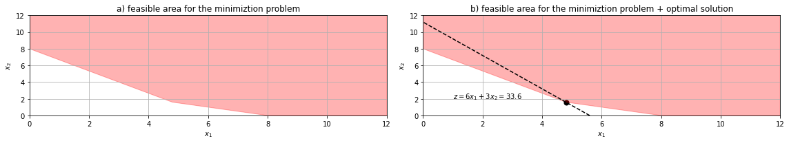
Minimization LP problems work similarly with contraints equations bearing the opposite inequlity sign. In example,

\[\begin{split} \begin{align} &\text{min}\\ &\qquad z=6𝑥_1 + 3𝑥_2\\ &\text{s.t.}\\ &\qquad 2x_1 + 4𝑥_2 \ge 18\\ &\qquad 4𝑥_1 + 3𝑥_2 \ge 24\\ &\qquad x_1, x_2\ge 0\\ \end{align} \end{split}\]

The solution can be found using the graphical method resulting in $(x_1,x2)=(4.8,1.6)$ and $z=33.6$.

import numpy as np
%matplotlib inline
import matplotlib.pyplot as plt
from matplotlib.patches import Polygon

plt.figure(figsize=(16,3))
#-------------------
plt.subplot(1,2,1)
P = np.array([
        [8, 12, 12, 0,  0, 4.8],
        [0,  0, 12, 12, 8, 1.6]
    ])
plt.gca().add_artist(Polygon(P.T, alpha=0.3, color="r"))
plt.grid()
plt.axis([0, 12, 0, 12])
plt.xlabel('$x_1$');plt.ylabel('$x_2$')
plt.title('a) feasible area for the minimiztion problem')
#-------------------
plt.subplot(1,2,2)
P = np.array([
        [8, 12, 12, 0,  0, 4.8],
        [0,  0, 12, 12, 8, 1.6]
    ])
plt.gca().add_artist(Polygon(P.T, alpha=0.3, color="r"))
plt.plot([33.6/6,0],[0,33.6/3],'--k')
plt.scatter(4.8,1.6,s=50,c='k')
plt.text(1,2, '$z=6x_1+3x_2=33.6$', color='k')

plt.grid()
plt.axis([0, 12, 0, 12])
plt.xlabel('$x_1$');plt.ylabel('$x_2$')
plt.title('b) feasible area for the minimiztion problem + optimal solution')
plt.tight_layout()
plt.show()

Surplus variables correspond to slack variables but represent an excess above a constraint requirement level. As with slack, surplus variables contribute nothing to the calculated value of the objective function. For the minimization problem, adding surplus variables results in,

\[\begin{split} \begin{align} &\text{min}\\ &\qquad z=6𝑥_1 + 3𝑥_2+0s_1+0s_2\\ &\text{s.t.}\\ &\qquad 2x_1 + 4𝑥_2 -s_1 = 18\\ &\qquad 4𝑥_1 + 3𝑥_2 -s1 = 24\\ &\qquad x_1, x_2, s_1, s_2\ge 0\\ \end{align} \end{split}\]

There are irregular types of LP problems for which the general rules do not apply. Particular kinds of issues include those with:

Multiple optimal solutions, i.e., the objective function is parallel to a constraint line.
Infeasible solutions, i.e., every possible solution violates at least one constraint.
Unbounded solutions, i.e., the value of the objective function increases indefinitely.

OR/MS in Python

Linear Programming¶

The Factory Problem¶

Graphical Solution of Linear Programming Models¶